Checking Whether or Not an Ad Is a Tide Ad with Keras And NumPy

Note : If you’re interested in machine learning, you can get a copy of my E-book, “The Mostly Mathless Guide to TensorFlow Machine Learning” by clicking HERE

There’s a bunch of kids running around with a Coca-Cola in their hands. But hold
on — look at their clothes! They’re so clean and white. Too clean, almost. Could this be a Tide ad?

Machine learning to the rescue! In this article, I’ll be showing you how to use TensorFlow, a machine learning library, to predict whether or not an ad is a Tide ad.

Prerequisites


This tutorial will be using Linux. You can probably do it on Windows too, but you may have to change some things. Here are the things you will need :

1. Python 3
2. TensorFlow (pip3 install tensorflow)
3. Keras (pip3 install keras)
4. ffmpeg (sudo apt-get install ffmpeg)
5. h5py (pip install h5py)
6. HDF5 (sudo apt-get install libhdf5-serial-dev)
7. Pillow (pip3 install pillow)
8. NumPy (pip3 install numpy)

Although VirtualEnv is not required, it is suggested that you use VirtualEnv to prevent any conflicts / version mistakes between Python 2 and Python 3.

Also, you can find all the code and bash scripts here : https://github.com/HenryDangPRG/TideAdIdentifier

Getting Started


First, we need to describe what our neural network will do. In this case, our neural network will will take one image as input, and tell you whether or not that image belongs to a Tide ad or not. Using ffmpeg, we can split a video into its frames to input an entire video into the neural network as well, and if over 50% of the frames in a video are classified as “Tide ads”, then we will consider it to be a Tide ad.

Next, we need data for our neural network to train on. The data will be a large set of .png images that we will get from slicing a video into individual pictures. I will not provide the videos as a download here, so you will need to find the 1 minute 45 second video of all the SuperBowl Tide ads, as well as 5 minutes worth of non-Tide ads. Also, the two videos should have the same size dimensions so that the images that come out are all the same size.

Once you obtain these two videos, convert them into .avi format and use ffmpeg to split them into its constituent frames. I’ve created a simple Bash script that will do the splitting process automatically for you, as long as you name the Tide ad video “tide.avi” and the non-Tide ad video “non_tide.avi”.

You can find the script here : https://github.com/HenryDangPRG/TideAdIdentifier/blob/master/generate_data.sh

The script above will take the two videos, and split 5 frames per second of the video, each frame being 512 x 288, into two separate folders. You can choose to do this on your own as well, but in this tutorial, as a convention, all Tide ad pictures will be in a directory called “tide_ads”, and all non-Tide ad pictures will be in a directory called “non_tide_ads”.

We’ll have to do the same with the test data, and the prediction data, and these are the bash scripts for those:

https://github.com/HenryDangPRG/TideAdIdentifier/blob/master/generate_test.sh
https://github.com/HenryDangPRG/TideAdIdentifier/blob/master/generate_predictions.sh

For the predictions, you can input any video format as the argument for the Bash script, but .avi is suggested for consistency.

NOTE : Remember to use chmod +x BASH_SCRIPT_NAME.sh on all of the Bash scripts so that you can execute them!

Creating A Convolutional Neural Network


Although this analogy is not perfect, you can think of a neural network as a group of students in a classroom who are all shouting out an answer. In this classroom, students are trying to determine whether or not a single image is from a Tide ad. Some students have a louder voice, so their “vote” for an answer counts more. A neural network can be thought of as thousands of students, all shouting different answers. The loudest answer gets passed to the next classroom, and those students discuss the answer (with their answers being modified by the previous classroom’s answer, perhaps by peer pressure), until we reach the very last classroom, where the loudest answer is the answer for the neural network.

201802081619561000

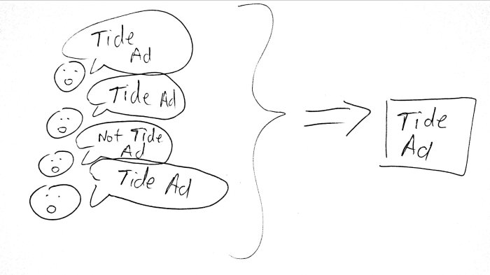
A convolutional neural network (CNN) is similar in that the students are still looking at an image, but they are only looking at a piece of the image. When they finish analyzing this image, they pass it to the next classroom, but the next classroom gets an even tinier piece of the original image. And so on and so forth, with each next classroom’s image getting smaller and smaller. When they’re done, a vote is outputted.

This is different in that in a normal neural network, the students vote for the entire image at once, but in a CNN, they each only vote for a piece of the image.

Now that you know the basics, let’s jump into the code.

Making The Magic Happen


First, let’s define the parameters for our CNN.

from keras.preprocessing.image import ImageDataGenerator
from keras.models import Sequential
from keras.layers import Conv2D, MaxPooling2D
from keras.layers import Activation, Dropout, Flatten, Dense
from keras import backend as K

# Could use larger dimensions, but will make training
# times much much longer
img_width, img_height = (128, 72)

train_dir = 'train_data'
test_dir = 'test_data'

num_train_samples = 4000
num_test_samples = 2000
epochs = 20
batch_size = 8

Each image will be shrunk to 128 x 72 pixels. Although we could go smaller, we would risk losing too much information. Larger could be better, but the larger the image dimensions are, the longer it will take for the CNN to train.

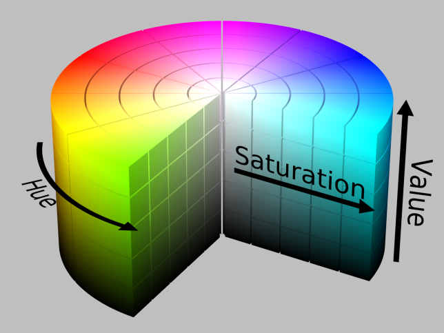
Next, we’ll have to specify in our CNN whether the color channels are first or last. Usually, they are first, though (at least, for png files). Note that an image could have just one color channel if it was grayscale, but in this case, we will only be using color images. We have to specify these because Keras will reduce our images into NumPy arrays, and the ordering matters.

# If data is formatted to have the channels first,
# then stick the RGB channels in front, else put them
# at the end.
if K.image_data_format() == 'channels_first':
    input_shape = (3, img_width, img_height)
else:
    input_shape = (img_width, img_height, 3)

Now that our CNN knows how many color channels (3 means RGB) our pictures have, as well as the dimensions of the image, we can apply three layers of convolution -> RELu -> max pooling.

The convolution step is essentially taking a tiny matrix and multiplying it to sections of the original matrix. When this is done, the result of each multiplication is recorded into a new matrix. The result is that we get a smaller matrix, which is called a feature map, containing unique features of the image that the machine can then process.

Next, we will need to apply ReLu, or Rectified Linear Unit. ReLu is incredibly simple. If the number is negative, make it zero, otherwise, leave it alone. This is because for a neural network, a negative value doesn’t really offer much information in the context of an image.

Imagine if we were detecting whether or not an image has dark blue lines. A value of zero in the feature map just means that there are no dark blue lines, while a positive value means that there might be a dark blue line. If so, then a negative value has no useful meaning, and can just be set to zero. ReLu also makes computations easier because zeroes are incredibly easy to deal with.

Finally, we apply max pooling, which takes subsections of a matrix and extracts the highest value from that subsection. This will shrink the matrix,reducing computation times, as well as giving us the most important parts of the matrix.

For our Tide ad predictor, we’ll use three layers of convolution, ReLu, and max pooling. When we’re done, we’ll put it all together with a fully connected layer.

# First convolution layer
model = Sequential()
model.add(Conv2D(32, (3, 3), input_shape=input_shape))
model.add(Activation('relu'))
model.add(MaxPooling2D(pool_size=(2, 2)))

# Second convolution layer
model.add(Conv2D(32, (3, 3)))
model.add(Activation('relu'))
model.add(MaxPooling2D(pool_size=(2, 2)))

# Third convolution layer
model.add(Conv2D(64, (3, 3)))
model.add(Activation('relu'))
model.add(MaxPooling2D(pool_size=(2, 2)))

# Convolution is done, so make the fully connected layer
model.add(Flatten())
model.add(Dense(64))
model.add(Activation('relu'))

Then, we apply dropout. Dropout, in our classroom analogy, is like duct taping certain students so that they cannot vote. By using dropout, every student needs to learn to give the right answer, rather than depending on the “smart” students to give the right answers. This gives us an extra layer of redundancy and prevents the loudest students from always overpowering the quiet students.

201802081702131000

In the context of neural networks, it stops overfitting, which is when the neural network becomes too accustomed to the training data and fails to generalize for data that it hasn’t seen before. This can be caused when certain neurons have their weights modified too much by the previous layer’s weights, especially when one neuron has an abnormally high weight. Dropout makes it so that the influence of any one neuron (or group of neurons) is significantly reduced.

From here, everything is pretty self-explanatory. We create some extra data points by slightly modifying the original images, and then plug those into our model. Finally, we train the data and save the completed CNN model.

# perform random transformations so that the
# data is more varied
train_datagen = ImageDataGenerator(
    rescale=1. / 255,
    shear_range=0.2,
    zoom_range=0.2,
    horizontal_flip=True)

test_datagen = ImageDataGenerator(rescale=1. / 255)

# make extra training data by modifying original training images
train_generator = train_datagen.flow_from_directory(
    train_dir,
    target_size=(img_width, img_height),
    batch_size=batch_size,
    class_mode='binary')

# make extra test data by modifying original test images
validation_generator = test_datagen.flow_from_directory(
    test_dir,
    target_size=(img_width, img_height),
    batch_size=batch_size,
    class_mode='binary')

# Train the CNN
model.fit_generator(
    train_generator,
    steps_per_epoch=num_train_samples // batch_size,
    epochs=epochs,
    validation_data=validation_generator,
    validation_steps=num_test_samples // batch_size)

# Saved CNN model for use with predictions
model.save('saved_model.h5')

If you don’t want to spend the time finding videos and training the CNN, the trained model is available in the GitHub repository here : https://github.com/HenryDangPRG/TideAdIdentifier

Predicting Whether a Video Is a Tide Ad


The prediction part is fairly trivial. All we need to do is take a video, turn it into image frames, turn those image frames into NumPy arrays, and then feed them into the trained CNN.

The video splitting part is done by generate_predictions.sh. All this Python code below does is feed those image frames into the CNN. If more than half of the frames aren’t Tide ads, then we can conclude that the video probably isn’t a Tide ad. (note that in the prediction array, a value of 1 means it is NOT a Tide ad, and a value of 0 means that it IS a tide ad)

import numpy as np
import subprocess
from keras.preprocessing import image
from keras.models import load_model

def img_to_array(file_name):
    loaded_img = image.load_img(file_name, target_size=(img_width, img_height))
    img_array = image.img_to_array(loaded_img)
    img_array = np.expand_dims(img_array, axis=0)
    return img_array

if __name__ == "__main__":
    directory = "predictions/"
    num_images = int(subprocess.getoutput("ls predictions | wc -l"))
    img_width, img_height = (128, 72)

    # load the saved model, and use it for prediction
    model = load_model("saved_model.h5")
    images = []

    for i in range(1, num_images+1):
        # Need up to 6 leading zeroes for formatting
        i_ = "{:0>7}".format(i)
        next_img = img_to_array(directory + "prediction-" + str(i_) + ".png")
        images.append(next_img)  
    images = np.vstack(images) 
    prediction = model.predict(images) 
    percent_tide = sum(prediction)[0] * 100 / num_images

    print("There is a " + str(percent_tide) + "% chance this is not a Tide ad.")

    # If more than half the images are NOT Tide ads
    if(sum(prediction) >= num_images / 2):
        print("It can be concluded that this is NOT a Tide ad!")
    else:
        print("It can be concluded that this IS a Tide ad!")

Conclusion


How well does this work? Well, not too well. This neural network uses a pitifully small data set, and was trained for very few epochs, so it makes sense that the results are not particularly accurate.

Inputting in Pepsi’s 2018 SuperBowl ad gives the following result :

There is a 45.833333333333336% chance this is not a Tide ad.
It can be concluded that this IS a Tide ad!

And inputting in Skittle’s 2018 SuperBowl ad gives this result :

There is a 53.4675615212528% chance this is not a Tide ad.
It can be concluded that this is NOT a Tide ad!

So, does this make every SuperBowl ad a Tide ad? Our neural network seems to think it does. Almost.

Common Boat Anchors in Programming and How to Avoid Them

A boat anchor is a metaphor that describes something that is obsolete or useless. In programming, boat anchors are everywhere. If you aren’t careful, boat anchors can ruin your productivity and cause confusion. Luckily, boat anchors are easy to prevent and correct if you look out for them. With just a little bit of foresight, you too can preserve your sanity.

TODO comments


Everyone’s used it. A seemingly innocent TODO comment. No harm done, since it’s just a little reminder for yourself right?

Wrong.

TODO comments are not only useless, but a productivity sink as well. Firstly, the “TODO” that you gave for yourself usually never gets done, as it’s buried in some function or class that you probably won’t even revisit for another week or two. Even if you do see the TODO, you’ll most likely ignore it as you’ll be too focused on your current task.

Secondly, TODO comments are bad because they waste the reader’s time. TODO comments belong in a Trello board or some other organizational system, not in your code base. No one wants to waste time reading about something that you should have/want to have done, but never got around to.

Commented Code


In this day and age, if your organization uses GitHub or some other form of version control, commented code is absolutely useless. This isn’t referring to commenting your code with useful English messages, but rather commenting out chunks of runnable code.

Commented code is essentially noise for the reader. If you push commented code to your repository because you think you might “need it later”, then you are ignoring the key purpose of version control.

Version control saves code. If you ever need that snippet of code that you deleted two months ago, it’s easily accessible. Don’t comment out code, or you’ll end up with hundreds and hundreds of obsolete lines of code.

Uncommented Code That Is Unused


Imagine you’ve written a utility class that calculates mortgages for you.

Suddenly, you’re told that the feature is scrapped, but that it might make a reappearance in the future.

Upon hearing that it might be used again in the future, you decide to leave the utility class in the code, since you might “need it later”. Once again, this goes back to the idea of version control. If it’s not relevant, and if it’s never used or referenced, then it doesn’t belong in your repository. Delete it.

Obsolete Documentation


Let’s say you have a nifty little method that method that divides every number in a list by 4.

def list_divide(list, dividend):
  """
  Divides every number in a list by a
  dividend and returns a new list with 
  the resulting numbers.
  """
  ret_list = []
  
  for num in list:
    ret_list.append(num/dividend)
  
  return ret_list

Suddenly, you remember about division by zero and quickly add a check to your function.

def list_divide(list, dividend):
  """
  Divides every number in a list by a
  dividend and returns a new list with 
  the resulting numbers.
  """

  if dividend == 0:
    print("Dividend must not be zero.")
    return

  ret_list = []
  
  for num in list:
    ret_list.append(num/dividend)
  
  return ret_list

Unfortunately, since you didn’t update the documentation, the docstring is now a lie. It doesn’t tell the user what the function actually does. There is no reference to division by zero in the docstring, causing the documentation to become a boat anchor.

Outdated documentation causes all sorts of issues for users. Luckily, this issue is easy to resolve. As a rule of thumb, if you add additional functionality to a function, document it. Even if you don’t like documentation, or if you think it’s tedious and pointless, do it anyway. You’ll save other programmers from headaches and wasted time.

Adding Ticket Numbers as Comments


Although not extremely common, some people feel the need to compulsively comment every change they make with a ticket number.

For example, you might see something like this :

#Added foobar function to resolve ticket 53
def foobar(num):
  #Fixes ticket 281
  if num == 0:
    print("Hello World!")
  elif num == 3:
    #Added because of ticket 571
    print(num/9)
  #Added else because of ticket 1528
  else:
    #Due to ticket 4713, changed to 'Goodbye World!' 
    print("Goodbye World!")

Before long, everything in your code will have a comment regarding a ticket.

If you are guilty of doing this, stop it. No one cares what ticket number the fix was in. Make the fix, commit, and push. All of the comments about tickets and issue numbers are utterly pointless and end up as unnecessary noise to the reader.

If you feel that the change is so strange or quirky that you absolutely must give some sort of background information, then write a comment. Making the reader search up a specific ticket to understand the code is a gigantic time sink, especially since most tickets have multiple comments. No one wants to read through all that text. Summarize it in a single comment and move on.

Storing Variables For No Reason


It’s a common practice for developers to do something along the lines of this :

def foobar(num):
  return num * 13

#Doing this
num = foobar(32)
print(num)

#As opposed to
print(foobar(32))

In this case, as long as “num” is not set to some wildly long function call, there is no reason to store it as a variable. In this case, foobar(32) is short, so it should be directly inputted into another function, rather than being set to a variable, and then inputted into the function.

Assigning it to a variable when the functional call is short tells the reader, “The variable num is important. It will be reused later in some way somewhere down the line.”

Not only that, but unnecessarily creating variables adds extraneous code for no good reason.

Conclusion


Boat anchors are everywhere in code. If you can avoid them, you will make not only your life easier, but everyone else’s as well. No one wants to waste time reading excessive code. Reading code is already difficult. Making your peers read more code than necessary hurts their productivity and makes coding an unpleasant experience.

So be a good person. Prune off the excess and correct the outdated. If you find any excessive code, then remove it. If the documentation is inaccurate or outdated, fix it. It might be a thankless job, but know that you’ll have made the world just a little brighter in the process.

Canny Edge Detection in Python with OpenCV

NOTE: Are you interested in machine learning? You can get a copy of my TensorFlow machine learning book on Amazon by clicking HERE

In my previous tutorial, Color Detection in Python with OpenCV, I discussed how you could filter out parts of an image by color.

While it will work for detecting objects of a particular color, it doesn’t help if you’re trying to find a multi-colored object.

For this tutorial, we will be using this basket of fruits.

fruitbasket

Let’s say we wanted to detect everything except for the table.

We could try and use color, but that would fail very quickly because all of the fruits are different colors. Since canny edge detection doesn’t rely on color, we can use it to solve our problem.

Canny Edge Detection


If I asked you to draw around the basket, you could easily do it.

But hold on, why is it possible for you to differentiate between the basket and the table?

The answer is that the basket has a different image gradient than the table.

To understand what I mean, take a look at the same image in black and white.

fruitbasket_blackwhite

Even without color, you can clearly see the edges of the basket and fruits because the gradients are vastly different at the edges.

Canny edge detection uses this principle to differentiate between edges. All edges have different gradient intensities than their surroundings. If two adjacent parts of the image have the same gradient intensity, then it wouldn’t be an edge as they would have the same hue and saturation.

Applying Canny Edge Detection


We will be loading the image in as a black and white photo. Images in black and white still have gradients, so it is still possible to differentiate between edges. As a rule of thumb, things tend to be much simpler when they are in black and white.

After we load the image, we need to apply canny edge detection on it.

import cv2
from matplotlib import pyplot as plt

def nothing(x):
    pass


img_noblur = cv2.imread('fruitbasket.jpg', 0)
img = cv2.blur(img_noblur, (7,7))

canny_edge = cv2.Canny(img, 0, 0)

cv2.imshow('image', img)
cv2.imshow('canny_edge', canny_edge)

cv2.createTrackbar('min_value','canny_edge',0,500,nothing)
cv2.createTrackbar('max_value','canny_edge',0,500,nothing)

while(1):
    cv2.imshow('image', img)
    cv2.imshow('canny_edge', canny_edge)
    
    min_value = cv2.getTrackbarPos('min_value', 'canny_edge')
    max_value = cv2.getTrackbarPos('max_value', 'canny_edge')

    canny_edge = cv2.Canny(img, min_value, max_value)
    
    k = cv2.waitKey(37)
    if k == 27:
        break

There are four arguments for cv2.Canny. The first one is your input image. The second and third are the min and max values for the gradient intensity difference to be considered an edge. The fourth is an optional argument which we have left blank.

If the fourth argument is set to true, then it uses a slower and more accurate edge detection algorithm. But by default, it is false and will calculate gradient intensity by adding up the absolute values of the gradient’s X and Y components.

Before canny edge detection can be applied, it is usually a good idea to apply a blur to the image so that random noise doesn’t get detected as an edge.

You can adjust the track bar however you’d like to edit the min and max values for the canny edge detection. I found that a min value of 36 and a max value of 53 worked well.

results

It also depends on how much you are blurring the image. The more you blur the image, the less noise there is. However, blurrier image have less accurate edges.

On the flip side, not enough blurring causes random noise to be detected. In the end, the level of blur is a trade-off between noise and edge accuracy.

Conclusion

Canny edge detection is only one of the many ways to do edge detection. There are hundreds of different edge detection methods, including Sobel, Roberts, SUSAN, Prewitt, and Deriche.

All edge detection methods have pros and cons, and Canny is just one of them. In general, canny edge detection tends to yield good results in most scenarios, so it is well-suited for general use. However, other edge detectors may be better depending on the situation.

If Canny isn’t working effectively for you, try a different solution. The best way to know if something works well is to test it out for yourself.

Why Keyword Arguments in Python are Useful

In Python, there are two types of arguments : Positional arguments and keyword arguments.

A positional argument is a normal argument in Python. You pass in some data as input, and that becomes your positional argument.

def foo(posArg):
  print(posArg)

There’s nothing unique or inherently special about positional arguments, but let’s say you have a function that evaluates your pet. Is your pet happy? Is your pet healthy? Is your pet playful?

def evaluatePet(isHappy, isHealthy, isPlayful):
  if(isHappy):
    print('Your pet is happy!')
  
  if(isHealthy):
    print('Your pet is healthy!')
 
  if(isPlayful):
    print('Your pet is playful!')

That’s fine and dandy, but what does it look like when we call the function?

 
evaluatePet(True, True, False)

We get the output :

Your pet is happy!
Your pet is healthy!

The result is correct, but the function call is absolutely unreadable.
A reader who has never read the documentation for evaluatePet will have a difficult time understanding what it does. From a quick glance, it takes three booleans. But what do those booleans describe? Whether it’s alive? Whether it’s a ghost? Whether it’s a flying ten thousand feet tall purple dinosaur?

The solution to this issue of readability is to avoid using a positional argument, and instead use a keyword argument.

A keyword argument is an argument that follows a positional argument, and allows the user to pass in arguments by explicitly stating the argument’s name, and then assigning a value to it.

In other words, you can call evaluatePet(True, True, False) in any of the following ways, without changing anything in the evalulatePet function.

#Explicitly calling the names and
#assigning all three of the arguments
evaluatePet(isHappy = True, isHealthy = True, isPlayful = False)

#Switching the order of the arguments.
#Since the arguments are named, 
#the order can be anything you like.
evaluatePet(isHealthy = True, isPlayful = False, isHappy = True)

#You can use positional arguments AND keyword arguments
#at the same time, as long as the keyword arguments
#are AFTER the positional arguments.
evaluatePet(True, isHealthy = True, isPlayful = False)

#Keyword arguments can ALWAYS 
#be switched around in any order
evaluatePet(True, isPlayful = False, isHealthy = True)

However, there are some things that you can’t do.

#Putting keyword argument before
#positional argument is illegal
#Will error, 
#"Positional argument follows keyword argument."
evaluatePet(isPlayful = False, isHealthy = True, True,) 

#Also will error for the same reason.
evaluatePet(isPlayful = False, True, isHealthy = True) 

You can see that with keyword arguments, the arguments are explicitly assigned. There is no confusion. The reader can simply look at a line like :

evaluatePet(isHealthy = True, isPlayful = False, isHappy = True)

And they will automtaically know, “Oh. This function takes in three booleans which are, isHealthy, isPlayful, and isHappy.”

It would be a huge understatement to say that this is the only thing that keyword arguments can do.

You can also load in defaults.

def evaluatePet(isHappy = False, isHealthy = False, isPlayful = False):
  if(isHappy):
    print('Your pet is happy!')
  
  if(isHealthy):
    print('Your pet is healthy!')
 
  if(isPlayful):
    print('Your pet is playful!')

Now, all three arguments become optional, and become automatically assigned to False if that specific argument has not been assigned.

#All three are automatically set to False, 
#so nothing is printed.
evalulatePet()

#You can set just one to True, 
#and the rest will automatically be False.
evaluatePet(isHappy = True)
evaluatePet(True)

Convenient, isn’t it? You can give your function a ton of default values, and then allow the user to change any defaults they don’t like, without requiring them to rewrite all the default values.

Underneath all of this magic, Python created a dictionary with a key value pair, where the keys are the argument names, and the values are the values you assign to those argument names.

If you want to prove this fact, you can use a true keyword argument by putting a double asterisk before an argument.

def foo(**kwargs):
  print(str(kwargs))

foo(bar = "henry", baz = "dang", foobar = "prg")

Output :

{'bar': 'henry', 'foobar': 'prg', 'baz' : 'dang'

In other words, Python has been converting evaluatePet’s arguments into a dictionary.

Naturally, Python wants the group of keyword arguments together, because it is cheaper to lump all the arguments together if they are all within one specific range (and not broken up between multiple ranges). In addition to this, Python can’t accept a positional argument after a keyword argument because it is impossible to determine which argument you are referring to. Are you referring to the first argument? Or the argument after the keyword argument?

These two reasons combined are why you can’t put in positional arguments, and then keyword arguments, and then another positional argument.

You might argue that Python should be able to do this :

evaluatePet(isHappy = False, isHealthy = False, False)

Since there are only three arguments, and two of them are keyword arguments, the third argument must be “isPlayful”.

However, Python’s philosophy is
“Special cases aren’t special enough to break the rules.”

So instead of Python automatically iterating over your arguments to figure out which argument hasn’t been assigned yet (you shouldn’t do this anyway since iterating over a list is expensive), Python simply says, “This is a special case. Follow the rules and deal with it.”

So while Python could potentially have allowed this special case to work, their mantra of sticking strongly to rules prevents you from doing so.

In a nutshell, keyword arguments are simply augments to Python’s core philosophy that “readability counts”. Without keyword arguments, readers must examine the documentation to understand what the arguments mean, especially if there are many arguments. The use of defaults also makes functions shorter if the user is unlikely to modify the defaults.

Shorter argument lists? Argument defaults? Understandable parameters? That’s elegant.

How URL Routing in Django Works

A URL is a uniform resource locator. It contains the address that links to a resource such as an HTML page.

For example, “https://henrydangprg.com” is a URL, that links to the HTML page that contains this website. A single website, like this, can have many other URL’s formed by adding a backslash (“/”) after the domain name.

If you wanted to access the about page on this website, you would add “/about/” to the end of the home page’s URL. It can be visualized like a tree.

You start with the base website, and you have other possible URL’s accessible by adding a backslash and some word.

  • https://henrydangprg.com/
    • about/
    • contact/
    • infinitely-many-other-possibilities/
      • which-can-contain-other-links/
        • containing-potentially-even-more-links/

In theory, you can have something like :

https://henrydangprg.com/foo/bar/foobar/foobarbar/foofoo-ad-infinitum/

How Does It Work in Django?

In Django, the premise is exactly the same. Inside each project is a urls.py file.

You’ll see something along the lines of this :

from django.conf.urls import url
from django.contrib import admin

urlpatterns = [
  url(r'^admin/', admin.site.urls),
]

Here, you can see that Django handles the URL routing with regular expressions. The ‘r’ before a string indicates that the following string is raw input. This means that Python will not convert things like ‘\n’ into a new line, and will instead process it as is.

You can play around with the urlpatterns list, and add new url’s to test that it works.

For example, if we change it to :

urlpatterns = [
  url(r'^admin/', admin.site.urls),
  url(r'^foobar/', admin.site.urls),
]

Then foobar will become a possible extension to your website’s URL. Assuming you’re using localhost and a port of 8000, it would be 127.0.0.1:8000/foobar/ to access your new URL.

If you want to go down two layers deep, like 127.0.0.1:8000/foobar/foo, you should create a new app.

Let’s make a new app called “foobar”.

django-admin startapp foobar

Modify the urlpatterns list inside your project’s urls.py file. We are now going to add foobar’s urls.py file into the project’s urls.py.

from django.conf.urls import include, url
from django.contrib import admin

urlpatterns = [
  url(r'^foobar/', include('foobar.urls')),
  url(r'^admin/', admin.site.urls),
]

Essentially, any time we visit 127.0.0.1:8000/foobar/, Django will see that we want to access “foobar”, and will check foobar’s urls.py for the next portion of the URL.

Now, we have to add add URLs into foobar. Go into the foobar directory and modify urls.py.

from django.conf.urls import url
from django.contrib import admin

from . import views

urlpatterns = [
  url(r'^$/', admin.site.urls),
  url(r'^foo/', admin.site.urls),
]

I don’t suggest you actually make every URL link to admin.site.urls, but for the sake of simplicity, we will stick to using that.

The ‘^$’ simply indicates that if there is nothing, then load the admin page. In this case, it would be 127.0.0.1:8000/foobar/ because there is nothing after “foobar/”, which is what our project’s urls.py looked up until.

We also added “foo” to our urlpatterns, which means we can now visit 127.0.0.1:8000/foobar/foo, allowing us to add extensions to our URL.

You can add virtually any URL you want, and as many levels of URLS as needed. You don’t even have to add new apps for each new extension. However, you will have to write a lot of duplicated code if you do that.


#With new apps 

urlpatterns = [
  url(r'^foobar/', include('foobar.urls')),
  url(r'^admin/', admin.site.urls),
]

#foobar.urls
urlpatterns = [
  url(r'^$/', admin.site.urls),
  url(r'^foo/', admin.site.urls),
]

#Without new apps, anti-DRY

urlpatterns = [
  url(r'^foobar/$', admin.site.urls),
  url(r'^foobar/foo$', admin.site.urls)
  url(r'^admin/$', admin.site.urls),
]

You can see that you would have to write out the full URL each time. If you had 100 URL’s, all 100 would have to be crammed into this single urlpatterns list, and if it goes 10 layers deep, you would have to write it all out each time.

Conclusion

URL routing with Django is absurdly easy, provided that you know a little bit of regex. However, if you are struggling with regular expressions, you can click here for an interactive regular expressions tester.
Best of luck with learning Django, and happy coding!


Five Great Practices for Safer Code

You’re sitting at your desk, glaring at your monitor, but it glares back at you with equal determination.

Every change you make introduces new bugs, and fixing a bug causes another bug to pop up.

You don’t understand why things are randomly breaking, and the lines of code just increase every day.

However, by coding in a rigorous and specific fashion, you can prevent many of these issues simply by being slightly paranoid. This paranoia can save you hours in the future, just by dedicating a few extra seconds to include some additional safeguards.

So without further ado, let’s jump right into the top five tips for safer code.

1. Stop Accepting Garbage Input


The common phrase “Garbage in, Garbage out” is one that rings strongly with many programmers. The fact is, if you accept garbage input, you’re going to pass out garbage output. If your code has any modularity at all, then something like this will likely happen :

def foo(input):
  do_stuff

def bar(input):
  do_other_stuff

garbage_input = 'Hi. I'm garbage input.'

some_variable = foo(bar(garbage_input))


As you call foo and bar and other functions, all of which depended on garbage_input, you find that everything has turned into garbage. As a result, functions will start throwing errors a few dozen passes down the line, and things will become very difficult to debug.

Another common mistake is attempting to correct the user’s input in potentially ambiguous cases, which leads to the second tip.

2. Don’t Try to Correct Garbage Input


Let’s take an example scenario :

Imagine you had a box that exported values from 0 to 1 on a display, depending on the number the user passed in.

One day, you suddenly get a value of 1.01, a value slightly higher than the maximum. Now, this should raise a red flag for most programmers. However, some programmers resort to doing the following :

def calculateValue(temperature):
  do_calculations

def getBoxValue(temperature):
  if calculateValue(temperature) > 1 :
    return 1
  elif calculateValue(temperature) < 0 :
    return 0
  else:
    return calculateValue(temperature)

The technique shown above is known as clamping, which is basically restricting the value to a certain range. In this case, it is clamped to 0 and 1. However, the problem with the above example is that it is now impossible to debug the code.

If the user passed in bad input, you would get a clamped answer, instead of an error, and if the calculateValue function was buggy, you would never know. It could be slightly inflating the value, and you would still never know, because the values would be clamped.

As an exaggerated example, if calculateValue returned 900,000,000, all you would see is “1”. Instead of embracing and fixing bugs, this tactic throws them under the carpet in the hopes that no one will notice.

A better solution would be :

def calculateValue(temperature):
  do_calculations

def getBoxValue(temperature):
  if(calculateValue(temperature) > 1
       or calculateValue(temperature) < 0):
    raise ValueError('Output is greater than 1 or less than 0.')
  else:
    return calculateValue(temperature)

If your code is going to fail, then fail fast and fix it fast. Don’t try to polish garbage. Polished garbage is still garbage.

3. Stop Double Checking Boolean Values in If Statements


Many programmers already adhere to this principle, but some do not.

Since Python prevents the bug caused by double checking a boolean value, I will be using Java, as the bug can only happen in languages where assignment is possible in if statements.

In a nutshell, if you do this :

boolean someBoolean = true;

if(someBoolean == true) {
  System.out.println('Boolean is true!');
} else {
  System.out.println('Boolean is false!');
}

In this case,

if(someBoolean == true)

Is exactly equivalent to :

if(someBoolean)

Aside from being redundant and taking up extra characters, this practice can cause horrible bugs, as very few programmers will bother to glance twice at an if statement that checks for true/false.

Take a look at the following example.

boolean someBoolean = (1 + 1 == 3);

if(someBoolean = true) {
  System.out.println('1 + 1 equals 3!');
} else {
  System.out.println('1 + 1 is not equal to 3!');
}

At first glance, you would expect it to print out “1 + 1 is not equal to 3!”. However, on closer inspection, we see that it prints out “1 + 1 equals 3!” due to a very silly but possible mistake.

By writing,

if(someBoolean = true)


The programmer had accidentally set someBoolean to true instead of comparing someBoolean to true, causing the wrong output.

In languages such as Python, assignment in an if statement will not work. Guido van Rossum explicitly made it a syntax error due to the prevalence of programmers accidentally causing assignments in if statements instead of comparisons.

4. Put Immutable Objects First In Equality Checks


This is a nifty trick that piggy backs off the previous tip. If you’ve ever done defensive programming, then you have most likely seen this before.

Instead of writing :

if(obj == null) {
  //stuff happens
}

Flip the order such that null is first.

if(null == obj) {
  //stuff happens
}

Null is immutable, meaning you can’t assign null to the object. If you try to set null to obj, Java will throw an error.

As a result, you can prevent the silly mistake of accidentally causing unintentional assignment during equality checks. Naturally, if you set obj to null, the compiler will throw an error because it’s checking a null object when it expects a boolean.

However, if you are passing around methods inside the if statement, it can become dangerous, particularly methods that will return a boolean type. The problem is doubly bad if you have overloaded methods.

The following example illustrates this point :

final int CONSTANT_NUM = 5;

public boolean foo(int x){
  return x%2 != 0;
}

public boolean foo(boolean x){
  return !x;
}

public void compareVals(int x){
  if(foo(x = CONSTANT_NUM)){
    //insert magic here
  }
}

In this example, the user expects foo to be passed in a boolean of whether or not x is equal to a constant number, 5.

However, instead of comparing the two values, x is set to 5. The expected value if the comparison was done correctly would be false, but if x is set to CONSTANT_NUM, then the value will end up being true instead.

5. Leave Uninitialized Variables Uninitialized


It doesn’t matter what language you use, always leave your uninitialized variables as null, None, nil, or whatever your language’s equivalent is.

The only exception to this rule is booleans, which should almost always be set to false when initialized. The exception is for booleans with names such as keepRunning, which you will want to set initially to true.

In Java’s case,

int x;
String y;
boolean z = false;

In particular, for Python especially, if you have a list, make sure that you do not set it to an empty list.

The same also applies to strings.

Do this :

some_string = None
list = None

Not this :

some_string = ''
list = []

There is a world of a difference between a null/None/nil list, and an empty list, and a world of a difference between a null/None/nil string, and an empty string.

An empty value means that the object was assigned an empty value on purpose, and was initialized.

A null value means that the object doesn’t have a value, because it has not been initialized.

In addition, it is good to have null errors caused by uninitialized objects.

It is unpleasant to say the least when an uninitialized string is set to “” and is prematurely passed into a function without being assigned a non-empty value.

As usual, garbage input will give you garbage output.

Conclusion


These five tips are not a magical silver bullet that will prevent you from making any bugs at all in the future. Even if you follow these five tips, you won’t suddenly have exponentially better code.

Good programming style, proper documentation, and following common conventions for your programming language come first. These little tricks will only marginally decrease your bug count. However, they also only take about an extra few seconds of your time, so the overhead is negligible.

Sacrificing a few seconds of your time for slightly safer code is a trade most people would take any day, especially if it can increase production speed and prevent silly mistakes.

Color Detection in Python with OpenCV

NOTE: Are you interested in machine learning? You can get a copy of my TensorFlow machine learning book on Amazon by clicking HERE

Image processing may seem like a daunting and scary task, but it’s actually not as terrible as some people make it out to be. In this tutorial, we will be doing basic color detection in OpenCV version 2.4.13. with Python 3.5. Note that you will also need to install NumPy to run the code in this article.

How Does Color Work on a Computer?


On a computer, color can be represented in many formats. However, in this tutorial, we will be strictly concerned with only BGR (Blue, Green, Red) and HSV (Hue Saturation Value).

With BGR, a pixel is represented by 3 parameters, blue, green, and red. Each parameter usually has a value from 0 – 255. For example, a pure blue pixel on your computer screen would have a B value of 255, a G value of 0, and a R value of 0. Your computer would read this and say, “Ah. This pixel is 255 parts blue, 0 parts green, and 0 parts red.”

With HSV, a pixel is also represented by 3 parameters, but it is instead Hue, Saturation and Value.

Unlike BGR, HSV does not use the primary color to represent a pixel. Instead, it uses hue, which is the color or shade of the pixel.

The saturation is the intensity of the color. A saturation of 0 is white, and a saturation of 255 is maximum intensity. Another way to think about it is to imagine saturation as the colorfulness of a certain pixel. Value is the simplest of the three, as it is just how bright or dark the color is.

HSV can be imagined like a three dimensional cylinder, as seen in the picture below.

hsv_color_solid_cylinder_alpha_lowgamma
Photo taken from Wikipedia’s HSL and HSV article.

Converting BGR to HSV


Since we will be using HSV, you will need an BGR to HSV to converter because OpenCV uses a different HSV scale from popular image editors like Gimp.

First, copy the following code into your favorite text editor and save it as converter.py. The lower and upper bound part will be explained later.

import sys
import numpy as np
import cv2

blue = sys.argv[1]
green = sys.argv[2]
red = sys.argv[3]  

color = np.uint8([[[blue, green, red]]])
hsv_color = cv2.cvtColor(color, cv2.COLOR_BGR2HSV)

hue = hsv_color[0][0][0]

print("Lower bound is :"),
print("[" + str(hue-10) + ", 100, 100]\n")

print("Upper bound is :"),
print("[" + str(hue + 10) + ", 255, 255]")

Now, we need an image to do color detection on. Download the image below and place it in the same directory as converter.py

circles

We have an image, and an BGR to HSV converter. That’s all we need to get started, so let’s jump into the actual image processing.

Let’s Get to the Code Already!


Fire up your favorite text editor and save a new file called “image.py” in the same directory as the circles.png file.

First, we need to grab our imports and load the image in OpenCV.

import cv2
import numpy as np

img = cv2.imread('circles.png', 1)

The 1 means we want the image in BGR, and not in grayscale.

As stated before, we will be using HSV instead of BGR, so we need to convert our BGR image to a HSV image with the following line.

hsv = cv2.cvtColor(img, cv2.COLOR_BGR2HSV)

Great! Now that the picture is in HSV, we need something called a “lower range” and an “upper range” for the hue that we are searching for. The lower range is the minimum shade of red that will be detected, and the upper range is the maximum shade of red that will be detected. In our case, let’s search for the red circle at the top left. To do so, we will need to obtain the RGB numbers for the red circle.

I personally prefer Gimp, so I will be using that for the color picker feature. Simply use the color picker and click on the red circle, and you will have copied it. Now, click on the red shade that you copied. (see photo below)

color-picker

After clicking on that, you should see the following screen :

color-bgr.png

We can see that red equals 237, green equals 28, and blue equals 36. We will be using these numbers with the converter to automatically generate the respective lower range and upper range HSV values for OpenCV. (Note that this method is inaccurate when the color is less pure or murky)

Remember that the HSV values shown in the photo are different from the ones in OpenCV. The scaling is different, so you can not use the values Gimp gives you for OpenCV.

Open up your terminal or command line and cd into the directory with the converter.py file and run the following :


python3 converter.py 36 28 237

Note that the order is in BGR, not RGB. After you run the script, it should output that the lower range = [169, 100, 100] and the upper range = [189, 255, 255].

We will now use NumPy to create arrays to hold our lower and upper range.

lower_range = np.array([169, 100, 100], dtype=np.uint8)
upper_range = np.array([189, 255, 255], dtype=np.uint8)

The “dtype = np.uint8” simply means that it will have the data type an 8 bit integer, which makes sense, because the max possible value for the hue, saturation, and value is 2^8 – 1.

Finally, with the lower range and the upper range found, we can create a mask for our image.

mask = cv2.inRange(hsv, lower_range, upper_range)

cv2.imshow('mask',mask)
cv2.imshow('image', img)

while(1):
  k = cv2.waitKey(0)
  if(k == 27):
    break

cv2.destroyAllWindows()

A mask is simply a specific part of the image. In this case, we are checking through the hsv image, and checking for colors that are between the lower-range and upper-range. The areas that match will be set to the mask variable.

After that, we can display both the mask and the image side-by-side.

The last three lines just state that the program will wait until the user presses the “esc” key (which has an id of 27) before it quits and destroys every OpenCV window.

If you’ve followed up to this point, you should end up with a mask that only has filled in white pixels for where the red circle was.

final-result

And there you have it! You just did color matching in OpenCV. We found an upper and lower bound for the shade of red that we were looking for, and created a mask that only had white pixels filled in for wherever there was a red that matched.

The next tutorial in this OpenCV series is Canny Edge Detection in Python with OpenCV.