The Illustrated Guide To Salting Passwords

This is Bob, the snail.

Bob just hacked your company’s authentication database, containing your customer’s secrets. Depending on how well you’ve secured those secrets, Bob either becomes a rich and happy snail, or he ends up getting nothing.

So let’s see what happens to Bob, based on how you stored your company’s secrets.

Level 0 – Plain Text

At level 0, it’s amateur hour. Your secrets are all stored in plain-text.

Your team is composed of literal monkeys who accidentally created a piece of software by mashing random buttons until they got a program that compiled.

Because you’ve stored all of the passwords in plain-text, Bob now has instant-access to all of your customer’s information. Not only that, since most people use the same password on several websites, he’s got access to those accounts as well.

Bob now gets to relax on the forest floor, while money showers down on him from all of the accounts he’s hacked.

Level 1 – Hashing

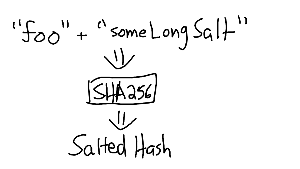
One step up from plain-text is basic hashing with SHA256. When you hash a string, you get another string as output. This output is always the same length, regardless of its input length.

Additionally, the hash function is irreversible, and doesn’t give you any useful indication about the input. In the example below, the SHA256 hash for “foo” and “fooo” are completely different, even though they are only one letter apart.

While hashes can’t be reversed, they can be cracked. All Bob has to do is bring out his trusty tool, the rainbow table.

You see, hashes have a problem, which is that they always produce the same output no matter what.

In other words, when I use SHA256 to hash “foo”, I always get “2c26b46b68ffc68ff99b453c1d30413413422d706483bfa0f98a5e886266e7ae” no matter what.

What Bob has done, is used something called a “rainbow table”, which is a table that contains input keys, and the hashed outputs for those keys (typically as chains of hashes).

Theoretically, if Bob had lots of storage space, Bob could generate all possible passwords up to 8 characters in length, hash every single of those passwords, and store them. Once Bob has assembled his rainbow table, Bob will be able to automatically crack any password hashed with SHA256 in the blink of an eye if it’s 8 characters or less.

Why? Because Bob has already pre-computed all the possible hashes for all 8 (or less) character passwords.

Realistically, Bob is bottlenecked by memory and computation times when it comes to how long his rainbow table can be. Let’s say passwords can contain alphanumerical characters (35 possibilities) and symbols that are located on a normal keyboard, like +, -, ~, \, etc. This gives us an additional 21 possibilities.

In reality, there are way more possible characters, but let’s say that there were 56 in theory as a lower bound. If Bob wants to generate all 5 character possibilities, Bob needs to generate 550,731,776 inputs, and hash all them.

Here’s a chart that shows how absurd the rate of growth is for rainbow tables (assuming 56 possibilities per character):

# characters# of generated inputs
156
3175,616
5550,731,776
896,717,311,574,016
10303,305,489,096,114,176 (303 quadrillion)
169,354,238,358,105,289,311,446,368,256 (9 octillion)

As you can see, rainbow tables really can’t extend very far. Eight characters is still feasible, but after that, it gets inordinately expensive. A 16-character rainbow table would be incredibly difficult to store, and would take an eternity to generate. Note that 56 characters is an incredibly low bound, since there are many other characters that can be used as well. You should expect it to be even more expensive, in practice, to generate a full rainbow table for all 1-8 character passwords.

Level 2 – Salt And Hash

Clearly, the problem with our previous approach was that we were hashing passwords, but these hashed passwords could be cracked by a rainbow table.

So how do we prevent rainbow tables from being used against us?

By using salts! A salt is just a simple string that, in many cases, is just appended to your password before it’s hashed. These salts are generally randomly generated and quite long (16+ characters), which means that our user’s password (8-16 characters) plus the salt (16 characters) should be at least 24 characters long (also note that every password should have a different salt).

This makes our unhashed password at minimum 24 characters, so this password can’t exist in a rainbow table because no one has the capability to generate all possible passwords up to 24 characters long.

We then hash this password, and store both the hashed + salted password, as well as the salt itself, in our database.

But what about our salt? It’s stored in plain-text!

The salt actually has to be stored in plain-text, because the way we verify a salted hash is that we take the user’s inputted password, append the salt, then hash it. If it matches what’s in our database, then it’s the correct password.

So how does all of this effect Bob? Well for starters, it makes the rainbow table incredibly useless. Although Bob has our salt, Bob can’t use his rainbow table against us, unless he re-generates an entirely new one, where each input has the salt appended to it.

For example, suppose our password was “foo”, and the salt was “saltyfish”. Without the salt, Bob would instantly be able to figure out the hash for “foo”. But with the salt, Bob now has to take all of his inputs, append “saltyfish” to them, and only then, will he find that “foosaltyfish” gives a hash match.

Once Bob finds the correct match, he removes the salt (“saltyfish”), leaving him with “foo”. And that’s our password! So Bob can still manage to hack our account.

But that was a really expensive operation. You don’t want to have to re-generate an entire rainbow table, because they’re often petabytes or larger in size. And the whole process of doing that only allowed you to hack one user! If Bob has to go through 300 million users, he would have to regenerate his rainbow table 300 million times, because every password has a different salt!

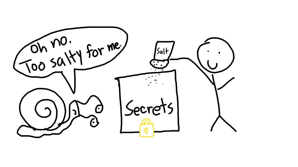
With your secrets safely salted, Bob has no choice but to find other unwitting victims to hack. Preferably, ones who haven’t salted and hashed their passwords.

Advertisement

The Illustrated Guide To Lazy Evaluation

Most people would tell you that hard work and perseverance are important if you want to be successful, but sometimes it pays to be lazy.

When it comes to programming, however, being lazy has plenty of benefits, and lazy evaluation is just one of those examples. Lazy evaluation is the idea of delaying the evaluation of an expression until the very moment in which you need it.

Lazy evaluation is most commonly used in functional programming languages, and the one of highest notoriety is Haskell, which is a completely lazy language by default (unless you tell it not to be)

How’s Lazy Evaluation Work?

Imagine that you’re a UPS (United Postal Service) employee and your job is to deliver some packages to your customer’s doorsteps.

Unfortunately, you are notoriously also the worst employee in your department.

Unlike a good employee, you don’t respect “Fragile” labels. In fact, you’re not even aware that the package is fragile at all. That’s why in the interest of time, you hurl every package you have, directly onto the hard, unforgiving concrete of your customers’s yards.

Do your packages make it in one piece? Who knows! You never look inside the box. For all we know, the box could be a bunch of stuffed animals, or it could be a very expensive $2,000 laptop that’s as fragile as a piece of glass.

As far as you are concerned, you have a box, and you transport it to someone else. This “box” is the expression, and evaluating the expression would be like opening the box to see its contents. While there is also metadata about the box, like whether it’s fragile or not, you have no clue whether it’s fragile or not until you read the information off the box.

Simply put, the essence of lazy evaluation is that you don’t know what’s inside something until you look at it. Initially, this sounds pretty simple and obvious. If you don’t look inside the box, how can you know what’s in it?

And that’s where it takes a loop. All of these boxes act like the box in Schrödinger’s cat experiment.

When it comes to lazy evaluation, you have no clue what’s in the box, but also there isn’t actually anything tangible in the box either. In a lazy evaluation model, to get a result out of the box, you would need to open it, and the very act of opening it causes the value inside to come into existence. Prior to opening the box, the box is essentially empty (an unevaluated expression, to be precise). It weighs nothing, makes no noise, and otherwise acts exactly like a normal box.

This can give us some pretty neat results. For example, suppose you have an expression like 1 divided by 0. This is the expression, which in our analogy, is the box. In a language like Python or Java, you would immediately crash with a divide by zero error.

But in Haskell, you can have an expression like “div 1 0”, and as long as you don’t evaluate it, nothing happens! You don’t get an error, because until you evaluate “div 1 0”, it simply exists as an expression with no value. Once you evaluate it (open the box, in this case), Haskell finds that the value is erroneous, and an error pops out.

Going a step further, what if you had a list that contained all of the numbers from 0 to infinity? (denoted as [0, infinity])

There is no doubt that this expression is infinite and contains all of the numbers from 0 to infinity. And yet, it doesn’t take up infinite memory, despite having an infinite size.

We can even take the first 5 terms out of this infinite list, and not crash. Why’s that? It’s because when you want to take the first 5 terms out, you evaluate only the first 5 terms in the list. As far as you are concerned, the other terms simply don’t exist, because you didn’t evaluate them into existence.

This means that you can pull finite results out of infinite lists, while also taking finite time and finite space. Note, however, that if you attempt to evaluate the entire list, it will end up taking infinite time, because each value of the list will materialize as each of the subexpressions get evaluated.

Consequently, if you tried to do anything like getting the length of the list, or trying to retrieve the last element in the list, you would not get a terminating result, because both of those require finding a final element, which doesn’t exist in the infinite list, and would require infinite evaluations to occur.

That sounds nifty and cool, but what about real-world applications?

If you’ve ever used a stream in any language (eg; Java streams), then you’ve used lazy evaluation. Streams, by nature, can be optimized by taking advantage of lazy evaluation.

In a real-world environment, streams can have millions to billions of elements. What if you wanted to concatenate two streams that each had at least 1 billion elements? Clearly, you can’t load either of the streams into memory, because that would quickly exceed memory limits.

This means you need to process the streams as abstract expressions, rather than as concrete values. Think of the streams as being two boxes, each containing potentially infinitely many items. With lazy evaluation, concatenating them together is a piece of cake — just put the two boxes inside of a new box.

At no point did you care about the insides of the stream, nor did you ever have to open the streams. This process has constant space and time complexity

With a non-lazy approach, you’d have to pull everything out of the second stream, find the ending element of the first stream, and then append each of the stream’s second elements one by one. Furthermore, you have to assume that no one adds any new elements into stream 1 as you’re appending the items in stream 2, which is a very big assumption to make. The reason the lazy approach doesn’t have this problem, is because you’re literally just stuffing the two streams into a new stream, without needing to know how many elements are in each of the streams, or what the elements are.

Conclusion

So with that, I hope you’ve gotten a better understanding of how lazy evaluation works. It has plenty of real-world use cases, and generally allows you to do operations on two, potentially infinite things, in constant time.

Lazy evaluation also allows you to defer errors until the very last moment, in which you have to evaluate an erroneous expression, at which point everything blows up. But if the erroneous expression is never needed (and thus never evaluated), then the error may as well not exist, which can be quite useful in some project workflows.

As a final note, lazy evaluation has some very notable drawbacks that you will need to be aware of. Firstly, if what you are doing is time-sensitive, like reading the current time, you will to immediately evaluate it on the spot.

This is because the “time” that you have is actually an expression that fetches the current time. The “current time” will actually be the time at which you evaluate it, and not the time at which the expression was created.

If you tried to time how long a program took to run by lazily fetching the start time, running the program, then lazily fetching the end time, you would find that both your start and end time are the same, and so it would output that the program took 0 seconds to run!

Hopefully, you’ve learned a bit about lazy evaluation from this article. There’s plenty more to learn about lazy evaluation, but the gist of it is that you can’t always use lazy evaluation.

As they old adage goes, sometimes, it pays to be lazy.